Creating business value from highly imbalanced datasets using mondrian conformal predictors

Updated on 9th Oct 2025

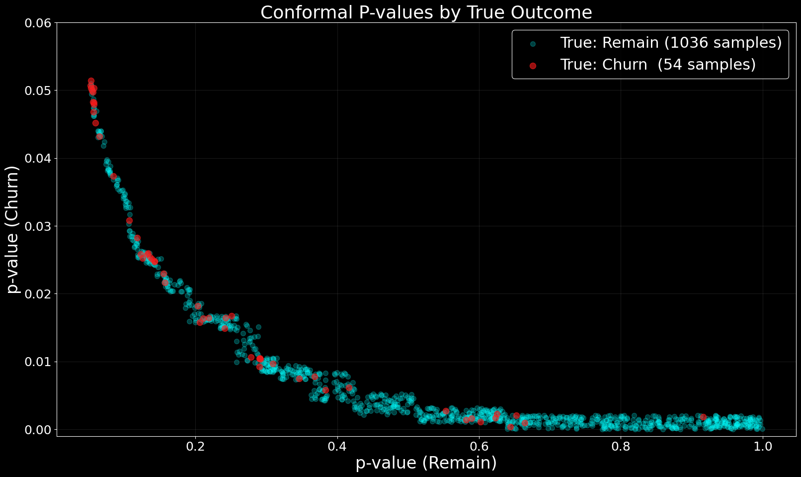
Recently, a customer offering a subscription service approached us with a churn case. The problem with churn cases is that the dataset tends to become highly imbalanced when we lower the time steps.

Assume a 20% YoY churn rate. We can potentially handle this scenario using traditional ML methods, smart feature engineering, and oversampling.

A 20% YoY churn rate equals 5% per quarter or 1.67% per month. Nasty imbalances!

Therefore, when we want to use last quarter’s churn data to predict the outcome for the next quarter, we have 5% churn to work with.

Takeaway: Balanced churn datasets indicate that the business experiences extremely high churn and are unlikely to survive.

In this post, I will recreate parts of our process for completing the task using a random public dataset.

You can find the code for this project on my GitHub.

The dataset

This public dataset describes a churn case for telecom customers and provides a good tabular dataset.

The dataset shows excessive balance compared to the customer case, with “only” 26.54% of customers churning. Therefore, I downsampled it to 5% churners to match quarterly models.

Models and data wrangling

To keep this light and easy, I have not done any feature engineering or more intimate data massaging. I’m keeping this recreation simple focusing on the imbalance rather than chasing the perfect score.

I also did not exclude a verification set since I did not perform any tuning. For our customer case, we developed the model using historical data and then ran the final model on the newest available data to prove the outcome.

The analysis uses all models with default settings and employs the raw dataset, with the churn class downsampled to 5%, without any feature engineering.

Naive random forest

We start by building a bog-standard random forest model. We perform no parameter tuning and make no model choice adjustments.

# Bog standard steps to choose target variable and 
# split dataset 80:20 train/test omitted 

clf = sklearn.ensemble.RandomForestClassifier(random_state=42)
clf.fit(X_train, y_train)

y_pred = clf.predict(X_test)
accuracy = sklearn.metrics.accuracy_score(y_test, y_pred)

Leading to this model outcome:

Target Churn Distribution:
     No: 95.01%
    Yes: 4.99%

Random Forest Classifier Results:
Accuracy: 0.9505

Classification Report:
              precision    recall  f1-score   support

          No       0.95      1.00      0.97      1036
         Yes       0.50      0.07      0.13        54

    accuracy                           0.95      1090
   macro avg       0.73      0.54      0.55      1090
weighted avg       0.93      0.95      0.93      1090


Churn Prediction Distribution:
  Predicted    No:  1082 (99.27%)
  Predicted   Yes:     8 (0.73%)

95% accuracy must be good, right?

Well. The model predicted that ~100% of customers would remain and caught ~0% of the customers who actually churned.

Enter Mondrian conformal predictors

Conformal predictors generate P-values for both outcomes: churn and remain. The Mondrian approach guarantees class-conditional coverage, ensuring valid prediction intervals for each target class separately.

We can therefore leverage the model’s uncertainty quantification to identify churners, as Mondrian conformal predictors provide valid coverage guarantees for both churners and remainers despite the massive class imbalance.

Beating through the dense statistical lingo we get the following properties:

Values on how well the sample matches both output classes due to knowing the prediction certainty.
We ensure coverage of both classes.

Perfect for a churn case with a class massive imbalance.

Requirements

We must withhold a calibration dataset to compute nonconformity scores for the Mondrian conformal predictor.
We must stratify the target class across the train/calibration/test split.

Outcome

The Mondrian conformal predictor generates p-values for both “remain” and “churn” classes when we predict on the test set.
We can utilize these p-values to optimize our true positive and false positive rates according to the business requirements.

The crepes package integrates traditional Scikit-Learn models with conformal prediction methods, including Mondrian conformal predictors. Those who want to explore the theoretical foundations in depth can find the corresponding papers linked in the repository’s citations section.

First, we split the data into train, calibration, and test sets. We stratify by the target class to maintain the same 95:5 remain-to-churn ratio across all sets. Since the class imbalance is extreme, any variation in class distribution will easily degrade model performance.

This stratification is particularly important for Mondrian conformal predictors, which compute class-conditional prediction sets and require consistent class distributions in the calibration set to ensure valid coverage guarantees for each class.

# First split: separate test set (20%)
X_temp, X_test, y_temp, y_test = sklearn.model_selection.train_test_split(
    X_array,
    y_encoded,
    test_size=0.2,
    random_state=42,
    stratify=y_encoded,
)

# Second split: divide remaining into train (62.5% of total) and  
# calibration (17.5% of total) 0.21875 of 0.8 = 0.175 of original
X_train, X_cal, y_train, y_cal = sklearn.model_selection.train_test_split(
    X_temp,
    y_temp,
    test_size=0.21875,
    random_state=42,
    stratify=y_temp,
)

We create a conformal classifier by wrapping the base random forest classifier.

clf = crepes.WrapClassifier(
    sklearn.ensemble.RandomForestClassifier(random_state=42)
)
clf.fit(X_train, y_train)

Calibration is trivial. mc=clf.predict enables the mondrian conformal prediction.

clf.calibrate(X_cal, y_cal, mc=clf.predict)

As a final step, we compute the p-values from the withheld test dataset.

p_values = clf.predict_p(X_test)

When we scatter plotting the confidence vs. true outcome we obtain a nice spread.

This is what enables us to create business value. We can quickly dismiss all data in the bottom right.

In the top left we have a cluster of certain churners.

Then we choose how many of the false positives in the middle we want.

If the activation cost for attempting customer retention is very low, then accepting more false positives will generate real positive business outcomes.

If the activation cost is high, we focus only on certain churners. Otherwise, we focus our attention elsewhere.

Conclusion

Mondrian conformal predictors enable us to move ahead despite facing previously near-insurmountable imbalanced datasets.

We perform no fine tuning or feature engineering in this recreation of the customer case. This establishes the baseline before we dig in, understand the dataset, derive more data about the customer, and then better inform the models.

With the P-values in hand, we can focus on business value and choose our desired outcome on the scale that encompasses all possible outcomes: false positives, true positives, false negatives, and true negatives.